The package h3 provides R bindings for H3, a hexagonal hierarchical spatial indexing system.
See also H3 Tutorial.
Core Functions
library(h3)

# Index a lat/lng point to an H3 index
coords <- c(37.5, -122.5)
res <- 9

(h3_index <- geo_to_h3(coords, res))
## [1] "8928342e20fffff"
# Get the center of an H3 index as a lat/lng point
h3_to_geo(h3_index)
## lat lng
## [1,] 37.50125 -122.5003
# Get the vertices of an H3 index as lat/lng points
h3_to_geo_boundary(h3_index)
## [[1]]
## lat lng
## [1,] 37.49974 -122.4990
## [2,] 37.50142 -122.4980
## [3,] 37.50293 -122.4992
## [4,] 37.50275 -122.5016
## [5,] 37.50107 -122.5026
## [6,] 37.49956 -122.5014Usually functions are vectorized:
(coords <- road_safety_greater_manchester[1:2, ])## lat lng
## 1 53.62111 -2.461070
## 2 53.61887 -2.458324
(h3_indexes <- geo_to_h3(coords, 8))## [1] "88195186b3fffff" "88195186b3fffff"
h3_to_geo_boundary(h3_indexes)## [[1]]
## lat lng
## [1,] 53.62557 -2.460912
## [2,] 53.62432 -2.467959
## [3,] 53.61988 -2.469062
## [4,] 53.61670 -2.463119
## [5,] 53.61796 -2.456073
## [6,] 53.62239 -2.454970
##
## [[2]]
## lat lng
## [1,] 53.62557 -2.460912
## [2,] 53.62432 -2.467959
## [3,] 53.61988 -2.469062
## [4,] 53.61670 -2.463119
## [5,] 53.61796 -2.456073
## [6,] 53.62239 -2.454970If sf is installed, you can get the polygons of H3 indexes like this:
h3_to_geo_boundary_sf(h3_indexes)## Simple feature collection with 2 features and 0 fields
## geometry type: POLYGON
## dimension: XY
## bbox: xmin: -2.469062 ymin: 53.6167 xmax: -2.45497 ymax: 53.62557
## CRS: EPSG:4326
## geometry
## 1 POLYGON ((-2.460912 53.6255...
## 2 POLYGON ((-2.460912 53.6255...Hierachy
# Get the children of an H3 index at the given (finer) resolution
(res <- h3_get_resolution(h3_index) + 1)
## [1] 10
h3_to_children(h3_index, res)## [1] "8a28342e20c7fff" "8a28342e20cffff" "8a28342e20d7fff" "8a28342e20dffff"
## [5] "8a28342e20e7fff" "8a28342e20effff" "8a28342e20f7fff"
# Get the parent of an H3 index at the given (coarser) resolution
(res <- h3_get_resolution(h3_index) - 1)
## [1] 8
h3_to_parent(h3_index, res)## [1] "8828342e21fffff"Traversal
# Find all H3 indexes within a given distance from the origin (filled ring)
radius <- 1
k_ring(h3_index, radius)
## [1] "8928342e20fffff" "8928342e20bffff" "8928342e273ffff" "8928342e277ffff"
## [5] "8928342e23bffff" "8928342e207ffff" "8928342e203ffff"
k_ring_distances(h3_index, radius = 2)## # A tibble: 19 x 2
## h3_index distance
## <chr> <dbl>
## 1 8928342e20fffff 0
## 2 8928342e20bffff 1
## 3 8928342e273ffff 1
## 4 8928342e277ffff 1
## 5 8928342e23bffff 1
## 6 8928342e207ffff 1
## 7 8928342e203ffff 1
## 8 8928342e21bffff 2
## 9 8928342e257ffff 2
## 10 8928342e247ffff 2
## 11 8928342e27bffff 2
## 12 8928342e263ffff 2
## 13 8928342e267ffff 2
## 14 8928342e22bffff 2
## 15 8928342e223ffff 2
## 16 8928342e233ffff 2
## 17 8928342e2abffff 2
## 18 8928342e217ffff 2
## 19 8928342e213ffff 2
# Get the distance in grid cells between two H3 indexes
h3_distance("8928342e20fffff", "8928342e21bffff")
## [1] 2Regions
# Get the multipolygon (array of polygons) for a set of H3 indexes
h3_indexes <- c("85291a6ffffffff", "85291a6bfffffff", "852834d3fffffff")
h3_set_to_multi_polygon(h3_indexes) %>%
  sf::st_geometry() %>% plot(col = "blue")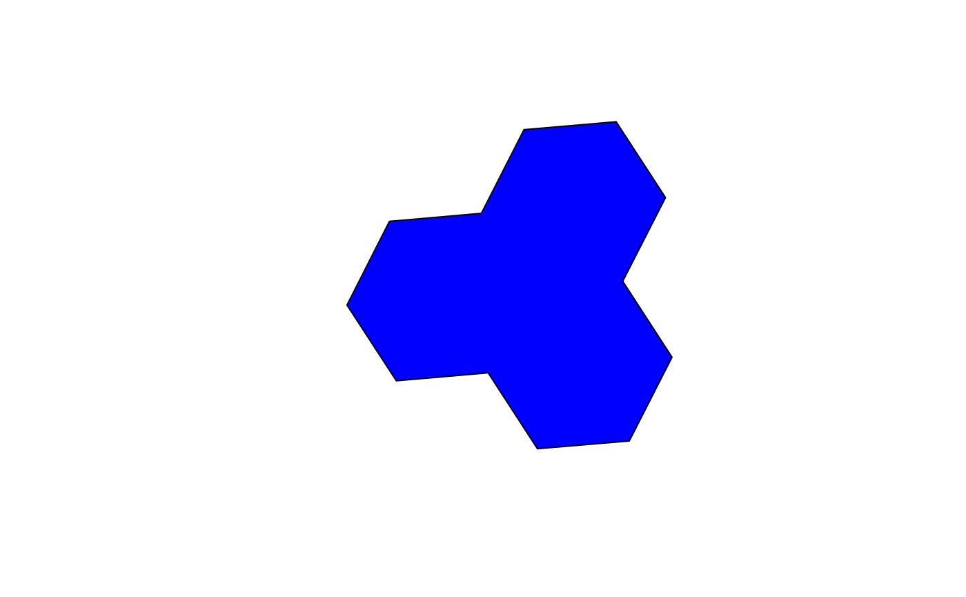
Rendering Hexagons
# Binning
h3_index <- geo_to_h3(road_safety_greater_manchester)
tbl <- table(h3_index) %>%
  tibble::as_tibble()
hexagons <- h3_to_geo_boundary_sf(tbl$h3_index) %>%
  dplyr::mutate(index = tbl$h3_index, accidents = tbl$n)
head(hexagons)
## Simple feature collection with 6 features and 2 fields
## geometry type: POLYGON
## dimension: XY
## bbox: xmin: -2.144701 ymin: 53.60199 xmax: -2.027979 ymax: 53.67943
## CRS: EPSG:4326
## geometry index accidents
## 1 POLYGON ((-2.083848 53.6794... 871942403ffffff 4
## 2 POLYGON ((-2.072919 53.6433... 87194240affffff 1
## 3 POLYGON ((-2.05044 53.62609... 87194240bffffff 1
## 4 POLYGON ((-2.061349 53.6622... 87194240effffff 1
## 5 POLYGON ((-2.129491 53.6587... 871942418ffffff 3
## 6 POLYGON ((-2.106978 53.6415... 871942419ffffff 3
# Rendering
library(leaflet)

pal <- colorBin("YlOrRd", domain = hexagons$accidents)

map <- leaflet(data = hexagons, width = "100%") %>%
  addProviderTiles("Stamen.Toner") %>%
  addPolygons(
    weight = 2,
    color = "white",
    fillColor = ~ pal(accidents),
    fillOpacity = 0.8,
    label = ~ sprintf("%i accidents (%s)", accidents, index)
  )

map